|
IV. CUBOCTAHEDRAL NUMBERS
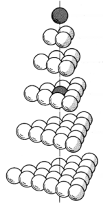
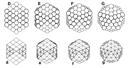
In the case of the cuboctahedron, the number of balls in successive shells
is 10 F^2 + 2, where F = 1,2,3... is the frequency of the shell,
i.e. number of between-ball intervals along an edge. The cuboctahedral
numbers would be running totals of the shells, plus the nuclear ball at
the center.
   shell=: (2&+) @ (10&* @ *:)  NB. 2 + 10* F^2

   shell >:i.10                 NB.  F = 1,2,3...
12 42 92 162 252 362 492 642 812 1002

   ] cuboctahedral =: 1,1 + +/\ shell >:i.10 NB. add nuke
1 13 55 147 309 561 923 1415 2057 2869 3871
The above series may be expressed more succinctly by evaluating the polynomial
(10/3)n^3 - 5n^2 + (11/3)n - 1, where n = 1,2,3... Let's
see this using rational number coefficients along with the polynomial
operator introduced in the previous lecture:
   poly =: _1 11r3 _5 10r3 & p.

   ] cuboctahedral =: poly >:i.11
1 13 55 147 309 561 923 1415 2057 2869 3871
The main reason for introducing the shells-based approach first, along with
the concept of frequency, was to make the link to geodesic spheres. Geodesic
spheres are often icosahedrally based, having 12 pentagonal hubs (vertices).
Their frequency is the number of struts (edges, intervals) between one
pentagonal hub and the next.
An icosahedral shell of frequency F has the same number of balls (vertices, hubs) as the corresponding cuboctahedral shell of the same frequency. Why this should be the case is dramatized visually by what R. Buckminster Fuller dubbed the "jitterbug transformation" whereby a cuboctahedral shell may transform into an icosahedral shell and vice versa.
The jitterbug transformation takes us from a polyhedron with 3 and 4-fold rotational symmetry (the cuboctahedron), to another polyhedron of five-fold rotational symmetry (the icosahedron).
Now that we've "jitterbugged" into the domain of five-fold rotational
symmetry, by distorting one of the cuboctahedron's shells, we may suppose
that we've left Pascal's Triangle behind, yet it comes up again in an
interesting way, in connection with the pentagon, the hallmark of this
five-fold world.
V. FIBONACCI NUMBERS AND THE GOLDEN MEAN
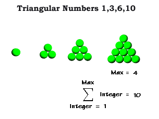
Recall that summing the terms of Pascal's Triangles along oblique diagonals
gives us the Fibonacci numbers.
   (i.11) { +/ /. pascal  NB. items 0,1..10 of oblique sums
1 1 2 3 5 8 13 21 34 55 89

   11 {. +/ /. pascal     NB. 11 {. gets the same thing
1 1 2 3 5 8 13 21 34 55 89

   pascal =: (nextrow ^: (i.21)) 1  NB. a bigger triangle

   fibos =: 21 {. +/ /. pascal  NB. more fibonacci numbers
   fibos = x: fibos  NB. convert to rational numbers (x:)
Taking the Fibonacci numbers in successive pairs, and dividing the larger
by the smaller, moves use ever closer to the golden ratio, known to the
greeks as phi, also equivalent to (1 + sqrt(5))/2.
That the Fibonacci numbers should converge to phi makes sense. 34 is
to 55 in about the same way 55 is to the whole (34 + 55 = 89), and this
whole is also the next Fibonacci number, and so on. This relationship
(of parts to wholes) gets more exact the further out we go.
   (1+%:5)%2   NB. phi =: (1 + sqrt(5)/2
1.61803
   55%34
1.61765
   89%55
1.61818
Phi is defined as a parts-to-whole relationship. Phi is the ratio of
two segments B, A such that the smaller (A) is to the larger (B), as the
larger (B) is to both combined (A+B). In other words, given A:B
= B:(A+B) then if A = 1, B = phi. The quantity (1 + sqrt(5))/2
may be computed directly from this equation.
In the section below, we study this convergence to phi, using a couple
more tricks around rational numbers and displayed precision (explained
below). This section uses the variable fibos defined
above: the first 20 Fibonacci numbers stored in rational form.
   ratios =: 2&(((1&{) % (0&{))\) NB. extract and divide
   ratios  NB. divide bigger by smaller in each group of 2


   5 4 $ ratios fibos  NB.  shape ratios into a 5x4 table
        1         2       3r2        5r3
      8r5      13r8     21r13      34r21
    55r34     89r55    144r89    233r144
  377r233   610r377   987r610   1597r987
2584r1597 4181r2584 6765r4181 10946r6765

   (9!:11) 12   NB.  !: invokes a "foreign" service (ouch)

   (x:^:_1) 5 4 $ ratios fibos  NB. convert to decimals
            1             2           1.5 1.66666666667
          1.6         1.625 1.61538461538 1.61904761905
1.61764705882 1.61818181818 1.61797752809 1.61805555556
1.61802575107 1.61803713528 1.61803278689 1.61803444782
 1.6180338134 1.61803405573 1.61803396317 1.61803399852

   ] phi =: 1r2 * 1 + x:%:5   NB.  phi as rational number

   phi
657194919625r406168797562     NB.  an approximation

   x:^:_1 phi                 NB.  the decimal version
1.61803398875
VI. INVERSE AND FOREIGN FUNCTIONS
We looked at x: in Lecture
One, and we know that ^:n is used to apply a function
n times. What we haven't seen before is getting an inverse function by
applying a function ^:_1 times. For example, the inverse
of squaring (*:) is the square root (%:),
and the powering operator makes this clear.
   square =: *:                NB.  name J's squaring verb
   squareroot =: (square ^:_1) NB.  same as %:
   square 10
100
   squareroot 100
10
Consistently, therefore, the inverse of x: is x:^:_1,
and its behavior is to convert a rational into a decimal.
Another feature of J is the large library of "foreign"
verbs, external to the language proper, and organized into numbered families
invoked with the dyadic conjuction !:.
These foreign verbs are used to read/write files, convert between data
types, get system time, memory statistics, or to toggle the display from
box view to tree view (something we've been doing via the GUI -- but could
just as well have done on the command line).
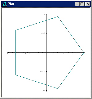
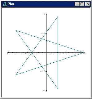
VI. PLOTTING A PENTAGON
Returning to our geometric explorations, the golden ratio (phi) describes
the ratio of any of the regular pentagon's five edges to any of the pentagon's
diagonals, which in turn describe a five-pointed star. We can show this
graphically, and then obtain phi by taking the ratio between a pentagon
edge and a star edge. The technique we use recaps what we did at the end
of Lecture One:
   (9!:11) 6            NB. display 6 digits of precision


   rotate =: 1ad72 & *  NB. 360 degrees divides into 5 x 72
   ] points =: +. rotate ^:(i.6) 1j0
        1            0
 0.309017     0.951057
_0.809017     0.587785
_0.809017    _0.587785
 0.309017    _0.951057
        1 _2.22045e_16

   pentx =: 0{"1 points  NB.  grab first column (x coords)
   penty =: 1{"1 points  NB.  grab 2nd column (=y coords
   pentagon =: pentx; penty
   load 'plot'
   plot pentagon

   starx =: 0 2 4 1 3 0 { 0{"1 points  NB. reordered points
   stary =: 0 2 4 1 3 0 { 1{"1 points
   star  =: starx; stary
   plot star


   'A B C' =: 0 1 2 { points   NB. take 3 points A,B,C
   distance =: %: @ +/ @: (*: @  -)  NB.  distance formula
'A B C' =: 0 1 2 { points NB. take 3 points A,B,C
distance =: %: @ +/ @: (*: @ -) NB. distance formula
Finally, I should explain this mystery of @: versus @
(@ inflected with a colon, vs. used alone). Let's look
at this distance formula in detail.
On the far right, we encounter the pattern (f@g), which, in a dyadic
situation, translates to f(g(x,y)). Remember our table from Lecture Two:
g(x,y)       <==> x g y         NB. simple dyadic form
f(g(x,y))    <==> x (f @ g) y   NB. dyadic g works on x,y)
So the subtraction operator gets used dyadically to subtract B from A,
and these are both 2-element arrays (x and y coordinates), so the result
is also a 2-element array.
   A
1 0
   B
0.309016994375 0.951056516295
   A-B
0.690983005625 _0.951056516295
*: then squares both (Ax-Bx) and (Ay-By) -- all a standard part of computing
distance. Notice that this technique would work just as well for 3-dimensional
coordinates, or more.
   *: A-B
0.477457514063 0.904508497187
Now comes the interesting part. If +/ were glued to
the squaring verb *: using @, it would
follow "atop" the squaring verb, tightly coupled to it, applying
immediately to each squared item.
But what we want is to apply +/ to the entire row, i.e. we want *: to
get through with its business and then use +/ to insert + between
its elements. This is where @: comes in: it says "allow
the action on the right to build up to as many dimensions as necessary,
and then eat it as a single whole" -- and in this case, "whole"
means a 1-dimensional array of numbers.
   +/ @ *: A-B      NB. +/ applies to each squared atom
0.477457514063 0.904508497187

   +/ @: *: A-B     NB  +/ applies to item of rank 1 (row)
1.38196601125
So the summation verb + adverb (+/)
adds both squared differences (or more, e.g. if we're in a 3-dimensional
coordinate system), giving back a single number, of which *:
then takes the 2nd root. So now we have our distances.
But do we have phi?
   (9!:11) 12  NB.  go back to 12 digit display

   (A distance C) % (A distance B)   NB. ratio = phi
1.61803398875
VII. PHI AS A CONTINUED FRACTION
Phi is also arguably the simplest of the non-terminating continued fractions,
with all coefficients = 1. J makes it easy to do continued
fractions, given its right-to-left execution mode.
The conventional expression:
1 + 1 /( 1 + 1 /(1 + 1 /(1 + 1/(1 + (1 + 1/(1 + 1/1))))))
is rewritten as:
(+ %) / 1 1 1 1 1 1 1
a hook which generatates
1 + %(1 + %(1 + %(1 + %(1 + %(1 + %1))))):
To summarize:
   1+1%(1+1%(1+1%(1+1%(1+(1+1%(1+1%1))))))   NB. dyadic %
1.63158

   1 + %(1 + %(1 + %(1 + %(1 + %(1 + %1))))) NB. monadic %
1.61538

   ( + %)/ 1 1 1 1 1 1 1  NB.  hook: (+ %) 1 = 1 + %1
1.61538

   (+ %) / 1 1 1 1 1 1 1 1 1 1 1  NB.  approximating phi
1.61797752809

   (+ %) / 20#1   NB.  apply to a list of 20 1s
1.61803399852

   (+ %) / 40#1   NB.  40#1 makes "40 copies of 1"
1.61803398875

   x:^:_1 phi     NB.  and there we have it!
1.61803398875
For further reading:
CP4E
|
2 +/\ 1 3 3 1 NB. monadic add insert (+/) gives sums 4 6 4
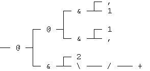
nextrow f. NB. changed configuration to tree view