Lecture Two:
Playing With Polynomials
by Kirby Urner
Oregon Curriculum Network
First posted: Sept 13, 2002
Last updated: Oct 10, 2002
I. POLYNOMIALS AND THEIR ROOTS
J includes a polynomial operator which accepts an array of coefficients on the left, and a value for x on the right. The coefficients map to increasing powers of x, not decreasing, as we typically expect in introductory algebra classes. In other words, 2 3 5 p. 3 means 2x^0 + 3x^1 + 5x^2, where x=3.
   2 3 5 p. 3   NB. evaluate, coefficients on left, x on right
56
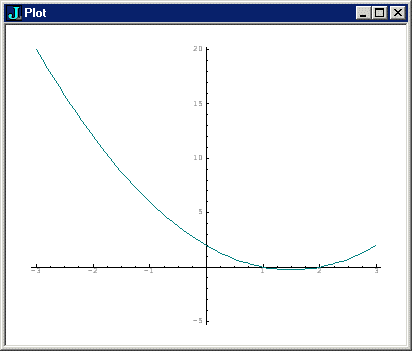
We might want to plot a polynomial by loading 'plot' and feeding it x and y coordinates.
   poly =: 2 _3 1 & p.    NB.  bond coefficients to p. = new verb
   range =: 0.1 * i:30    NB.  from _3 to 3 in increments of 0.1
   load 'plot'            NB.  load J-supplied plot scripts
   plot range;poly range  NB.  plot x,y

Notice the graph appears to intersect the x axis at (0,1) and (0,2). These would be the roots or zeros of our polynomial. Using p. monadically, with coefficients on the right, returns the zeros for that polynomial.
   p. 2 _3 1                 NB.  return roots of 2 -3x + x^2
+-+---+
|1|2 1|
+-+---+
The first box contains coefficient of the highest power, i.e. is the same as last non-zero coefficient in the array. The second box contains approximate roots, which may well be complex numbers.
The number of roots is the same as the degree of the polynomial, which is one less than the number of coefficients. Now let's get some roots and feed them back into the original polynomial, while shaping the results into more easily digested tables.
coeffs  =: 1 _2 3 _4 5       NB.  1 - 2x + 3x^2 - 4x^3 + 5x^4
roots =: 1 { > p. coeffs     NB.  roots from unboxed (>) results

   (4 1) $ roots             NB.  shape roots into a 4 x 1 table
 _0.137832j0.678154
_0.137832j_0.678154
  0.537832j0.358285
 0.537832j_0.358285

   (4 1) $ coeffs p. roots   NB.  use roots as values of polynomial
 2.22045e_16j8.32667e_17
2.22045e_16j_8.32667e_17
          0j_1.66533e_16
           0j1.66533e_16
As you can see from the large negative exponents, plugging the zeros of our polynomial back into the polynomial nets us values very close to zero, yet not exactly zero, as an iterative approximation method (such as LaGuerre's) had to be used internally.
When we multiply two polynomials together, we always get another polynomial -- same when we add. Polynomials form a ring, meaning we have closure under addition and multiplication (among other properties), but not under division: polynomials do not necessarily have multiplicative inverses that are themselves polynomials (we call them "rational expressions" in the general case).
II. DIFFERENTIATING AND INTEGRATING
Polynomials are also closed under integration and differentiation. Integrating and differentiating polynomials is easy, and is one of the first topics covered in beginning calculus. However, once the concepts are understood, and the process mastered, it's nice to have a computer do the grunt work.
p.. used as a monad differentiates a polynomial, given a list of coefficients on the right. p.. used as a dyad integrates, with the left argument being a constant of integration, i.e. that +C we add to the output of any integral.
   p.. 1 3r5 9r17 _7r10   NB. differentiate (rationals)
3r5 18r17 _21r10

   0 p.. 1 3r5 9r17 _7r10 NB. integrating same poly, add constant 0
0 1 3r10 3r17 _7r40
J also has the power to differentiate a polynomial starting not with its coefficients, but with its multiplier and roots. Compare the results based on both kinds of input:
   coeffs   =: 1 _2 3 _4 5  NB.  1 - 2x + 3x^2 - 4x^3 + 5x^4

   rootsbox =: p. coeffs    NB.  get the multiplier and roots

   p.. rootsbox             NB.  differentiate using the results
_2 6 _12 20

   p.. coeffs               NB.  using original coefficients
_2 6 _12 20
III. BOXING ELEMENTS AND TABULAR DISPLAYS
When we multiply two polynomials A and B, every coefficient in A multiplies every coefficent in B, and resulting terms are grouped by like powers. If we put the coefficients of A down the left side of a table, and coefficients B across the top, then we can look at the degrees of the resulting products by simply adding the powers of the left and top terms.
J lets us construct a Cartesian product of all pairs in a domain around any dyadic verb d0. The result of dyadically applying d0/ (a dyadic verb modified by /) is to return an array of A x B elements, where we have A along the first axis, and B along the next. The result of performing d0 on each (a,b) occurs in the corresponding row and column. For example, let d0 =: + (addition).
   d0 =: +

   0 1 2 3  d0/ 0 1 2 3 4
0 1 2 3 4
1 2 3 4 5
2 3 4 5 6
3 4 5 6 7


   d1 =: */
   (i.4) d1 i.4
0 0 0 0
0 1 2 3
0 2 4 6
0 3 6 9


   d2 =: !/             NB. dyadic ! = n!k means n!/k!(n-k)!
   (i.4) d2 (i.4)
1 1 1 1
0 1 2 3
0 0 1 3
0 0 0 1

   (i.10) d2 (i.10)     NB.  bigger table of binomial coefficients
1 1 1 1 1  1  1  1  1   1
0 1 2 3 4  5  6  7  8   9
0 0 1 3 6 10 15 21 28  36
0 0 0 1 4 10 20 35 56  84
0 0 0 0 1  5 15 35 70 126
0 0 0 0 0  1  6 21 56 126
0 0 0 0 0  0  1  7 28  84
0 0 0 0 0  0  0  1  8  36
0 0 0 0 0  0  0  0  1   9
0 0 0 0 0  0  0  0  0   1


   |: (i.10) d2 (i.10)  NB. use transpose (|:) to flip this around
1 0  0  0   0   0  0  0 0 0
1 1  0  0   0   0  0  0 0 0
1 2  1  0   0   0  0  0 0 0
1 3  3  1   0   0  0  0 0 0
1 4  6  4   1   0  0  0 0 0
1 5 10 10   5   1  0  0 0 0
1 6 15 20  15   6  1  0 0 0
1 7 21 35  35  21  7  1 0 0
1 8 28 56  70  56 28  8 1 0
1 9 36 84 126 126 84 36 9 1
The last expression generates what's known as Pascal's Triangle, alternatively the binomial coefficients of (1 + x)^n where n = 0,1,2...
If you want to see such tables with rows and columns included, not just the results, you may use the pre-defined adverb table as handy shorthand. table makes use of the boxing operator (<). The idea of a boxed array is very important in J. Boxes are what allows us to mix unlike nouns, for example integers and letters, in a single array. The dyadic ; concatenates heterogenous items into an array of boxes, as shown below:
  1 ; 'a' ; i. 2 2    NB.  box 1, 'a' and a 2x2 table
+-+-+---+
|1|a|0 1|
| | |2 3|
+-+-+---+
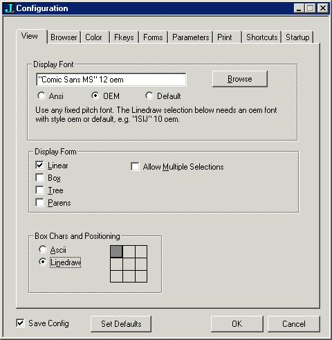
The use of ASCII characters to delineate boxes is somewhat unattractive, but is easiest to share, via web pages or email for example. If you want to have smoother lines when doing computer projector presentations in front of your class, this preference may be set in the configuration window.

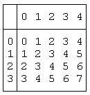
Let's use the table adverb to reformat the above addition table:
0 1 2 3 + table 0 1 2 3 4 NB. table modifies + (is an adverb)
IV. MULTIPLYING POLYNOMIALS
Now if we think of these consecutive integers as the powers of x in a polynomial, we see that like powers group obliquely. For example, the twos slant upward from the lower left to the middle top.
So if we first multiply all pairs of coefficents, then sum the oblique diagonals of the resulting table, we will effectively be summing all terms of like powers, ending up with the coefficients of the final polynomial.
A =: 1 _3 4 NB. coefficients of polynomial A B =: 2 1 _2 NB. coefficients of polynomial B A */ B NB. multiplication table of all (a,b) pairs 2 1 _2 _6 _3 6 8 4 _8 </. A */ B NB. box (<) oblique diagonals of A */ B+//. A */ B NB. instead of boxing, sum the diagonals (+/) 2 _5 3 10 _8 mp =: +//.@(*/) NB. capture all this in a single dyadic verb A mp B NB. mp means 'multiply polynomial' 2 _5 3 10 _8
The key observation to make regarding mp above is that it's a composition of two verbs: f =: +//. and g =: */ where */ is used dyadically.
In other words, the left and right arguments land on either side of */ to generate a multiplication table, and then +//. sums this table's oblique diagonals.
V. COMPOSING FUNCTIONS
This is a case where the conjuctions & and @, used as function composers, part company. They've had essentially the same meaning as long as both the conjoined verbs were monadic, but here the pattern x f @ g y is being interpreted as f (x g y), which is a description of @'s job.
   f =: +//.    NB.  used monadically to sum oblique diagonals
   g =: */      NB.  use as a dyad to built multiplication table

   1 _3 4 (f @ g) 2 1 _2
2 _5 3 10 _8
Were we to use & in place of @, then
the intepretation would be to treat g as the monad, applied
to both arguments. f would be the dyad. In other words,
the pattern would be
   g 2 1 _2     NB.  /* means 'insert *' between all items
_4


   g 1 _3 4
_12


   _12 f _4     NB.  +//. ignores left argument
_4

   1 _3 4 (f & g) 2 1 _2
_4
In beginning algebra, we learn to write f(g(x)) and g(f(x)) as "compositions of functions". However, this notation implies f and g are both monadic. Suppose g is dyadic. Then we might write: f(g(x,y)) g(f(x),f(y)) g(f(x),y) or g(x,f(y)).
J gives us all these function templates and more:
g(x,y)           <==> x g y         NB. simple dyadic form
f(g(x,y))        <==> x (f @ g) y   NB. dyadic g works on x,y
g(f(x),f(y))     <==> x (g & f) y   NB. dyadic g works on f(x),f(y)
g(f(x),y)        <==> (f x) g y     NB. f applies to x only
g(y,f(y))        <==> (g f) y       NB. monadic hook (no x)
g(x,f(y))        <==> x (g f) y     NB. dyadic hook
f'(g(f(x),f(y))  <==> x (f &. g) y  NB. f' is the inverse of f
We can even get a third function into play, plus make both f and g dyadic:
g(f(y),h(y))     <==>   (g f h) y   NB. monadic fork
g(f(x,y),h(x,y)) <==> x (g f h) y   NB. dyadic fork
And lets not forget the possibility that both f and g are monadic:
f(g(x))          <==> (f & g) x     NB. composing monadics
f(g(x))          <==> (f @ g) x     NB. same as above
f'(g(f(x))       <==> (g &. f) x    NB. f' is the inverse of f
What's especially useful about most of the above cases is that the verbs appear together, within parentheses, perhaps joined by a conjunction. These parenthetical patterns therefore serve as a basis for building verbs from other verbs, with no mention of the arguments.
The only exception to the rule was
g(f(x),y) <==> (f x) g y <==> x ((f @ [) g ]) y
Using the above patterns, we have the power to define generic verbs as compositions of other verbs, with no use of arguments x and y, even as placeholders. We'll only need specific arguments when we actually apply the verbs.
Don't feel you must commit all these patterns to memory in one fell swoop -- or ever, if your goals as a J user are on the modest side. You will gradually learn the patterns you most need.
When learning to compose verbs, it's probably easiest to start with simple monadic compositions, as we were doing with i&>: in Lecture One. In future, we'll see examples of other patterns. We'll also see that both & and @ may be inflected with the colon, which gives each a slightly different meaning having to do with their "rank" (see Lecture Three).
These so-called tacit definitions consisting of verbs, conjunctions and adverbs, all strung out on a single line, are concise, yet have their limitations. Tacit definitions, especially lengthy ones, also presume a certain comfort level with the language that comes with experience.
J permits a more conventional style of programming as well. Explicit definitions, may be multi-line, contain control structures such as loops, and bring the placeholder nouns x. and y. into the verb's definition. These stand for left and right arguments respectively.
VI. BINOMIAL COEFFICIENTS AND PASCAL'S TRIANGLE
Now that we have a verb for multiplying polynomials, we can generate the coefficients of (x+1)^n:
   binmult =: 1 1 & mp  NB.  bond coefficients 1 1 to multiplier
   binmult 1            NB.  (1 + x) * 1 = 1 + x
1 1

   binmult 1 1          NB.  (1 + x)(1 + x) = 1 + 2x + x^2
1 2 1

   binmult 1 2 1        NB.  = 1 + 3x + 3x^2 + x^3
1 3 3 1

   binmult 1 3 3 1      NB.  coefficients of (1 + x)^4
1 4 6 4 1

   (binmult ^: 10) 1    NB.  repeat application of binmult 10 times
1 10 45 120 210 252 210 120 45 10 1
And so we have another way of generating Pascal's Triangle:
   (binmult ^: (i.>:10)) 1  NB.  Applying binmult 0,1,2,...10 times

1  0  0   0   0   0   0   0  0  0 0
1  1  0   0   0   0   0   0  0  0 0
1  2  1   0   0   0   0   0  0  0 0
1  3  3   1   0   0   0   0  0  0 0
1  4  6   4   1   0   0   0  0  0 0
1  5 10  10   5   1   0   0  0  0 0
1  6 15  20  15   6   1   0  0  0 0
1  7 21  35  35  21   7   1  0  0 0
1  8 28  56  70  56  28   8  1  0 0
1  9 36  84 126 126  84  36  9  1 0
1 10 45 120 210 252 210 120 45 10 1
Now let's take the sums of Pascal's Triangle along oblique diagonals. We'll only take those diagonals which have a 1 in the left column:
   p =: (binmult ^: (i.>:10)) 1  NB. as above

   11 {. +//. p    NB. grab 11 sums (+/) of oblique diagonals (/.)
1 1 2 3 5 8 13 21 34 55 89

