|
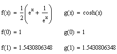
Necklaces, overhead telephone lines, anything string-like,
hanging from two ends with a dip in the middle owing to the pull of
gravity, will tend to assume this catenary shape.
On the other hand, when the chain or rope supports the weight of
something pulling down evenly along its entire length, like a road
bed, in the case of a suspension bridge, then the result is a
parabola.

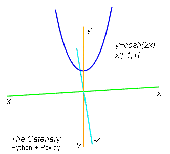
The above graphic was developed using Python + Povray, a generic computer
language (i.e. Python), and a specialized ray tracing engine with
scripting language (i.e. Povray) -- both multi-platform, free
downloads.
The functions.py source code
includes a primitive
mkdomain function for returning a list of domain values,
from low to high, in constant increments -- (low, high, step) being
the 3 parameters passed to this function.
Here's mkdomain in action:
>>> from catenary import *
>>> domain = mkdomain(-1,1,0.1)
>>> domain
[-1.0, -0.9, -0.8, -0.7, -0.6, -0.5, -0.4, -0.3, -0.2, -0.1,
0.0, 0.1, 0.2, 0.3, 0.4, 0.5, 0.6, 0.7, 0.8, 0.9, 1.0]
The catenary
function gets passed as a rule to mkfunction,
along with an optional value for k (which defaults to 1), so that
the range values cosh(kx) may be computed for every member
of the domain list.
defcatenary(x,k=1):
    return math.cosh(k*x)
The catenary function returns a list of (domain,range)
pairs i.e. a list of tuples. This is what a function amounts to,
after all; a function is a set, with each domain value uniquely
paired with some corresponding range value, more than it is some
rule or algebraic expression.
The list of tuples returned by catenary, in turn serves as grist
for the mill -- this time for the graphfunc utility.
In this function, we take successive (domain,range) points and draw
segments connecting them. If the points are close enough together,
the locally straight edges nevertheless provide a smoothly curving
result. This is how we got the curve shown above.
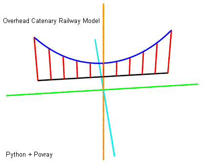
In the case of an overhead caternary railroad, a lower line is
suspended from an upper one, and charged with high voltage. This
line is then pressed against by the pantograph, that part of a
train which makes contact with the overhead wire.
In the real world, these might not really be catenary curves --
but these overhead wires are called
catenaries, in any case.
Of course it might be useful to figure out how long when of
these hanging dips might be. What is the length of a catenary? What
is the length of any arc? One solution, given we're doing these
Python functions, would be to accumulate the lengths of the little
segments we're using to connect the dots:
defgetlength(myfunc):
    """
    approximates length of curve as sum of segments
    for list of (x,f(x)) tuples
    """
    length = 0
    for i in range(len(myfunc)-1):
        v1 = Vector((myfunc[i]+(0,)))
        v2 = Vector((myfunc[i+1]+(0,)))
        length = length + (v2-v1).length()
    return length
In other words, we're already taking (domain,range) pairs and
drawing little segments between successive v1, v2. So
let's just write a take the cumulative sum of these lengths and see
what we get:
>>> from functions import *
>>> domain = mkdomain(-2,2,0.01)
>>> function = mkfunction(domain,catenary,{'k':2.0/3.0})
>>> getlength(function)
4.6476237334964479
>>> domain = mkdomain(-1,1,0.01)
>>> function = catenary(domain,catenary,{'k':2.0})
>>> getlength(function)
6.1125198957092381
Notice that it matters how closely together we space our domain
points. The closer together they are, the more closely our little
segments follow the curve itself.
This is a classic example of where the
calculus comes in handy, as clearly there's a limit case, where
we've gone as far as we can towards bringing our domain points
closer together. Using the calculus, we can compute this limiting
expression directly, without approximating through a sequence of
closer and closer values.
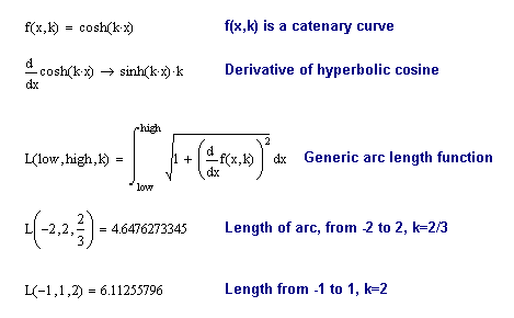
The calculus expression for arc length is given below: with low
and high values bracketing our domain, we integrate a 2nd root of
(1 plus the 2nd power of the derivative function). Given we can
take the derivative of cosh(kx), we have an expression for
arc length.

Notice that L(-2,2,2/3) gives a value rather close to what we
got using Python, as does L(-1,1,2).
Below we apply the same general approach to obtaining the arc
length using a semi-circle instead of a catenary. First, lets
specify the function in Python (invoking the already-supplied semicircle rule)
and add up all the little segments between successive tuples:
>>> from functions import *
>>> domain = mkdomain(-1,1,0.0001)    # passing low, high, interval
>>> semicirc = mkfunction(domain,semicircle)
>>> getlength(semicirc)
3.1415923595933619
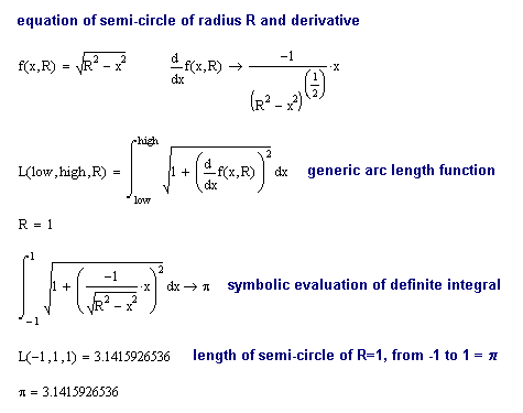
And here's the calculus approach, which nets us the expected
result of pi, for the length of a semi-circle with a radius
of 1 and a domain of [-1,1]. Note that our discrete math approach
in Python came pretty close, given the fine calibration of our
increments.
We also have a method for computing the tuples of the
derivative of some function -- i.e. the (domain, range) pairs
of another function. This method wiggles each domain value x
by ± h (a parameter), and computes the ratio of the
change in f(x) per change in x -- which value approaches
the derivative function's value at x, as h becomes
arbitrarily small.
This derivative function (a set of tuples) may be fed to
getlength1, which uses a discrete math version of the above arc
length integral, with delta x in place of dx. The
value of delta x should be the same as the interval used to
compute the original domain.
Below, the
mkderiv and
getlength1 methods are applied to a semi-circle. We use the
middle section, from -root(2)/2 to root(2)/2, to avoid troublesome
boundary conditions associated with a domain going all the way from
-1 to 1.
>>> from functions import *
>>> low = -2**0.5/2.0; high = -low
>>> domain = mkdomain(low,high,0.00001)
>>> deriv  = mkderiv(domain, semicircle, h=0.000001)
>>> part   = getlength1(deriv,0.00001) # note: same as interval
>>> 2 * part  # multiply by 2 to get full length of semi-circle
3.1416108619768579
The approximations for length obtained in this way are not as
good as using getlength, which in turn falls short of the
precision attained by the calculus approach (which depends on
symbolic, versus discrete numeric methods to compute the derivative
function).
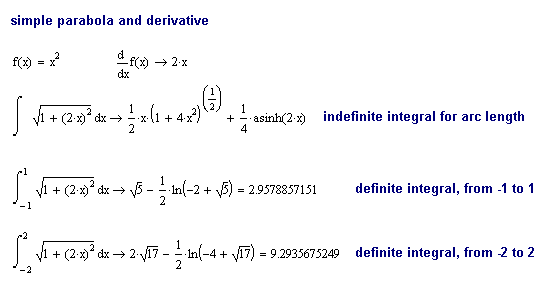
Finally, saving the best curve (or at least one of the most
popular) for last, we compute the arc length of a parabola over a
couple of intervals: [-1,1] and [-2,2]. Note that our indefinite
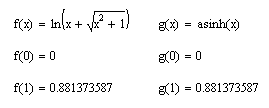
integral for arc length contains the hyperbolic arcsine function
(which may be expressed using Ln as shown below).
|
