1: Getting Serious About Series

by Kirby Urner
First posted: Feb 13, 2000
Last modified: Jan 7, 2003


One hallmark of the Oregon Curriculum Network approach is its focus on spatial geometry. For example, in this essay, I emphasize the following math facts:

  • various number series correspond to specific sphere packing arrangements
  • a square number is the sum of two consecutive triangular numbers
  • the sum of consecutive icosahedral shell numbers is a cuboctahedral number
  • triangular, square, and tetrahedral numbers show up in Pascal's Triangle
  • Pascal's Triangle connects to the golden ratio (phi) via the Fibonacci numbers
  • the golden rectangle is embedded in the icosahedron

Given this geometric focus, students will naturally want to do some modeling. Hands-on projects will of course require supplies of various kinds:

image

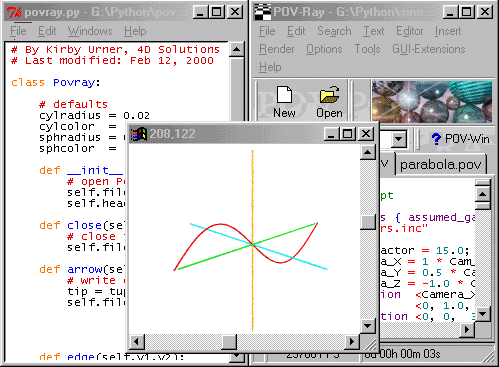
When it comes to computer graphics, we also need to supply some hardware and software tools. One promising approach (the one used in this essay) is to harness the combined power of:

  • Python, a free, cross-platform computer language with development environment
  • Povray, a free, cross-platform ray tracing package, plus scripting language
  • HTML, a cross-platform markup language for making text and graphics browsable
imagePython is not confined to performing in a graphics-related role in this curriculum, but serves as a general purpose workhorse. Python notation provides an alternative, human-readable syntax for various core algorithms (some going back hundreds or even thousands of years), thereby capturing the whole idea of "rules" and "rule following" (using Wittgenstein's terminology) -- with the computer (not the student-programmer) in the role of "mindless rule follower".

By supplementing conventional, pre-computer math notations with a very high level language (VHLL), we give students access to complementary modes of encoding rules. The hope is that students will learn to write programs as a means to test and refine their understanding of math concepts -- will look at programs as "math poems" (or as attempts toward this ideal).

The Python language (named for Monty Python, the British comedy troupe -- although the snake connotation gets some air play as well) is vastly more comprehensible to human readers than most other languages (e.g. C/C++), plus it provides an interactive, responsive environment giving students fast, positive reinforcement for correct usage.

For example, here's a simple rule for generating the triangular numbers:

 def tri(n):
    # triangular num n 
    # = sum of n consecutive counting nos (n>=1)
    if n<=1: return n
    else: return n + tri(n-1)  

The above rule, or function definition (def) returns the nth triangular number, and is defined recursively, meaning it calls itself repeatedly, until done.

And here's what it looks like to use this, and related functions, at the interactive command line:

Python 1.5.2 (#0, Apr 13 1999, 10:51:12) [MSC 32 bit (Intel)] on win32
Copyright 1991-1995 Stichting Mathematisch Centrum, Amsterdam
IDLE 0.5 -- press F1 for help
>>> import series
>>> series.tri(10)
55
>>> series.sqr(5)
25
>>> series.tetra(6)
56
>>> series.fibo(10) # the L identifies a "long integer" (potentially huge)
55L
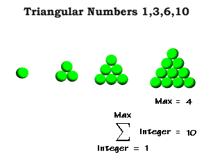
Triangular numbers are a kind of figurate number, meaning they're associated with geometric shapes.

If we have N spheres, and N is a triangular number, then these spheres may be shaped into a triangle with the same number of spheres to a side, as shown at right.

Each successive row contains one additional sphere, so the nth triangular number is likewise the sum of the first n positive integers.

image


But is this the only rule we might use to generate the triangular numbers? No. For example, we might simply use the expression ( (n+1) x n)/2 for the nth triangular number.

Or, to put it in Python:

def tri2(n):
    # triangular num n = sum of n consecutive counting nos
    return n*(n+1)/2

How is it that this alternative rule gives triangular numbers?

At this juncture, it's useful to share a story about the young Johann Carl Friedrich Gauss (1777-1855) , later a famous mathematician. The class was misbehaving and the teacher assigned everyone to find the sum of all the numbers from 1 to 100 as busy work.

The young Gauss, already brilliant, wrote two lines and added them, like this (notice we skip actually writing and adding most of the numbers -- so did he):

      1 +   2 +   3 + ... + 100
    100 +  99 +  98 + ... +   1 <-- same 100 terms in reverse 
    --------------------------- 
    101 + 101 + 101 + ... + 101 

Clearly, he reasoned, I'm getting this number 101 in the bottom row 100 times. But that's from adding all the numbers I need twice (I added the series to itself). So the number I really want is 1/2 of 100 x 101 = 10100/2 = 5050.

So a more general way of writing the solution is:

     1 +   2 +   3 + ... +   N 
     N + N-1 + N-2 + ... +   1 <-- same N terms in reverse 
   --------------------------- 
   N+1 + N+1 + N+1 + ... + N+1 

where we're adding all consecutive integers from 1 up to N. In other words, we have N+1 added to itself N times, for a total of N x (N+1). But again, that's from adding the series twice (adding it to itself). So the answer we're really looking for is:

Sum of N consecutive integers = N x (N+1) / 2

The sum of N consecutive integers is what we've already identified as triangular numbers. So this story about Gauss provides a derivation of this alternative rule.

Notice that two consecutive triangular numbers give a square number. Here's a simple geometric proof of that fact, in the form of "ASCII art":

  * * * * * *            * * * * * *      *   * * * * *   *   * * * * *
  * * * * * *          * * * * * *      * *   * * * *    * *   * * * *
  * * * * * *        * * * * * *      * * *   * * *     * * *   * * *
  * * * * * *  =   * * * * * *   =  * * * * + * *   =  * * * * + * * 
  * * * * * *    * * * * * *      * * * * *   *       * * * * *   *
  * * * * * *  * * * * * *      * * * * * *          * * * * * *

    SQR(N)                                         TRI(N) + TRI(N-1)

So we have the option to generate square numbers using the following rule, which makes use of the already-defined tri function:

def sqr(n):
    # square num = sum of 2 consecutive triangular nos
    return tri(n) + tri(n-1)    

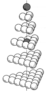
The sum of consecutive triangular numbers gives a tetrahedral number. The figure at right shows 6 triangular sphere packings, one atop the other. These layers collapse down to form a tetrahedron with a grand total of 1+3+6+10+15+21=56 spheres.

Again, we might go with a recursive definition:

def tetra(n):
    # tetrahedral num 
    # = sum of n consecutive triangular nos
    if n <= 1: return n
    else: return tetra(n-1) + tri(n)

Notice the previous function, tri(n) is part of the definition. This function counts all the spheres in the nth triangular layer, plus all the spheres in a tetrahedron of one fewer layers. Asking for the next smaller tetrahedron causes the function to invoke itself, and so on down to the very first sphere, at which point the looping stops and allows the function to return a cumulative sum.

image

Adapted from Fig 419.30 in
Synergetics by RBF


We need not confine ourselves to such recursive solutions however. Why not simply add consecutive triangular numbers in a simple (non-recursive) loop? Certainly this is a solution many students will consider the most straightforward:

def tetra2(n):
    # tetrahedral num = sum of n consecutive triangular nos
    sum = 0
    for i in range(1,n+1):
        sum = sum + tri(i)
    return sum

We also have a couple of short cuts to the nth tetrahedral number that bypasses summing a lot of consecutive triangular numbers (the For Further Reading section links to a derivation):

def tetra3(n):
    # tetrahedral num = sum of n consecutive triangular nos    
    return (1.0/6.0)*n*(n+1)*(n+2)

def tetra4(n):
    # tetrahedral num = sum of n consecutive triangular nos
    f=n-1  #using frequency as the variable 
    return (1.0/6.0)*f**3 + f**2 + (11.0/6.0)*f + 1

Just as triangular layers may be stacked to form a growing tetrahedron, so may square layers be stacked to form a growing half-octahedron, reminiscent of a Mayan Pyramid. These half-octahedral numbers will be sums of consecutive square numbers.

def hoct(n):
    # half octahedral num = sum n of consecutive squares
    if n <= 1: return n
    else: return hoct(n-1) + sqr(n)

Of central interest to the philosopher-architect R. Buckminster Fuller (1895-1983) were the icosahedral shell numbers, as these give the number of hubs in his geodesic spheres.

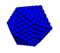
An icosahedral shell contains 10f2 + 2 spheres, where f stands for frequency and is the number of between-sphere intervals along any edge. For example, the 5-frequency icosahedral shell shown at right contains 252 spheres.

image

At the Python command line below, the argument is the number of spheres along an edge -- one more than the number of intervals (or frequency).

>>> series.icoshell(6)
252
>>> map(series.icoshell,[1,2,3,4,5,6,10])
[2, 12, 42, 92, 162, 252, 812] 

Given viruses tend to have an icosahedrally shaped protective shell, this number series also shows up in virology: "All of these numbers are in fact found in actual viruses, 12 for certain bacteriophages, 42 for wart viruses, 92 for reovirus, 162 for herpesvirus, 252 for adenovirus and 812 for a virus attacking crane-flies (Tipula or daddy-long-legs)" - The Natural History of Viruses by C.H. Andrews (W.W. Norton R Co., 1967).

image


How did we get the expression 10f2 + 2 for the number of spheres in an icosahedral shell? One way to arrive at this result is to realize that, because an icosahedron consists of 20 identical triangular faces, we must be adding the same triangular number tri(n) 20 times -- except then we must subtract from this total to balance for multiple counting.

After multiplying tri(n) by 20, every corner sphere -- of which there are 12 --will have been counted 5 times, i.e. 4 times too many. So subtract 4 x 12 = 48. And every non-corner edge sphere -- of which there are 30 * (n-2) -- will have been counted twice. So subtract this number as well.

In other words, another expression for icoshell would be:

def icoshell2(n):
   # alternative function for nth icosa shell number
   return 20*tri(n)-30*(n-2)-48

If you substitute f+1 for n in the above equation -- remembering to use the expression n(n+1)/2 for tri(n) -- you will get 10f2 + 2.

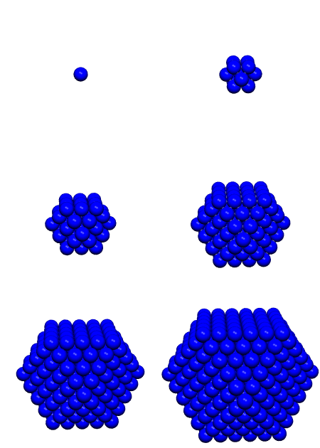
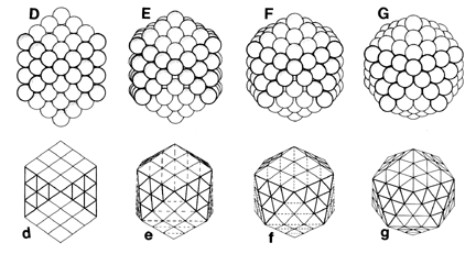
The icosahedron does not fill up with equi-radius spheres (not enough room), so it tends to be hollow. The cuboctahedral shell, on the other hand, contains the same number of spheres as the icosahedral shell, and it fills with equi-radius spheres in concentric layers.

We can see why icosahedral and cuboctahedral shell numbers are the same by considering how the cuboctahedron and icosahedron transform (or "morph") into one another.

image

Fig. 466.00a from RBF's Synergetics

imageThe sphere packings depicted above (top row) go from a cuboctahedral to an icosahedral conformation as we move from left to right. Beneath the sphere packings, we see the same transformation using edges and vertices -- the vertices correspond to the spheres in the row above. The number of spheres (or vertices) remains unchanged as we move from D (d) to G (g). This transformation is a phase of what Fuller dubbed "the jitterbug".
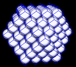
So a cuboctahedral number is the sum of consecutive icosahedral shell numbers -- with the first term in the series being 1 -- the nuclear sphere itself.

def icoshell(n):
    # number of spheres in an icosahedral shell 
    # if n spheres along an edge
    f= n-1
    return 10*f**2 + 2

def cubocta(n):
    if n<=1: return 1
    return icoshell(n) + cubocta(n-1)

And yes, there's an alternative function for cuboctahedral numbers, an equation in the third degree, a derivation of which is provided on a linked web page -- also see the series.poly function below.

def cubocta2(n):
    return (10.0/3.0)*n**3 - 5*n**2 + (11.0/3.0)*n - 1

The cuboctahedral sphere packing plays an important role in both science and architecture. Its sphere centers define the "face centered cubic lattice" (fcc), which is important in crystallography. In architecture, this lattice, or space frame, is called the "octet truss", and was studied by Alexander Graham Bell (1847-1922), among others.

Every sphere not on the edge of the packing is surrounding by twelve others. Each sphere may be inscribed inside a rhombic dodecahedron, a space-filling shape, such that all neighboring spheres are intertangent at the dodecahedron's face centers. Johannes Kepler (1571-1630) did a lot of pioneering studies in this area.

image


From these various number series and corresponding sphere packing arrangements, we now turn to Pascal's Triangle, named for Blaise Pascal (1623 - 1662), and also known to the Chinese.

Pascal's Triangle might be considered one of the "grand central stations" in our math curriculum, considering how many topical threads converge to it.


For example, we know that the young Isaac Newton (1642-1727) discovered a rule for generating the coefficients of (a + b)n, when expanded into a polynomial. We call this the Binomial Theorem. These same coefficients likewise appear in row n of Pascal's Triangle.

image


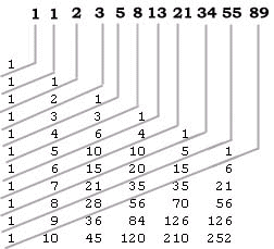
Notice the entries in each subsequent row may be obtained by adding one or two entries in the previous row: the entry in the same column plus the entry in the previous column (if there is one).

                                  1
                                1   1
                              1   2   1
                            1   3   3   1
                          1   4   6   4   1
                        1   5  10   10  5   1
                      1   6  15  20   15  6   1

Notice also that the sum of the terms in row n+1 is double the sum in row n. This makes sense in light of the fact that each term in the previous row contributes twice to the row below, once to the left, and once to the right -- an effective doubling of each term.

In the output below (shown in blue), the "L" after each number designates these as "long integers", meaning they have the capability to expand to many more digits than are normally expressible by an ordinary integer data type. This distinction is more relevant and familiar to computer scientists than mathematicians, but that's no reason for dropping it here, as the 'numeracy + computer literacy' approach seeks to hybridize these disciplines, in search of a stronger, more resilient genetic mix.

>>> series.prow(10)    # 10th row of Pascal's Triangle (row 0 = apex = 1)
[1L, 10L, 45L, 120L, 210L, 252L, 210L, 120L, 45L, 10L, 1L]
>>> series.sumprow(10) # = 2**10
1024L
>>> series.prow(11)
[1L, 11L, 55L, 165L, 330L, 462L, 462L, 330L, 165L, 55L, 11L, 1L]
>>> series.sumprow(11) # double the previous sum = 2**11
2048L

Especially interesting in the context of this discussion, is the fact that triangular and tetrahedral numbers appear in Pascal's Triangle as per this linked exhibit.

>>> series.showpascal(9)  # rows 0-9 (i.e. 10 rows in all)
[1]
[1, 1]
[1, 2, 1]
[1, 3, 3, 1]
[1, 4, 6, 4, 1]
[1, 5, 10, 10, 5, 1]
[1, 6, 15, 20, 15, 6, 1]
[1, 7, 21, 35, 35, 21, 7, 1]
[1, 8, 28, 56, 70, 56, 28, 8, 1]
[1, 9, 36, 84, 126, 126, 84, 36, 9, 1]

Notice the 3rd column in the above data: 1,3,6,10,15... triangular numbers. And in the 4th column we find the tetrahedral numbers. Therefore, if we have an algorithm to generate the individual entries of Pascal's Triangle (which we do, thanks to the Binomial Theorem), then we have yet another way to get triangular and tetrahedral numbers: we simply look them up by row and column number.

def ptri(n):
    # lookup nth triangular number in pascal's triangle
    return pascal(n+1,n-1)
    
def ptetra(n):
    # lookup nth tetrahedral number in pascal's triangle
    return pascal(n+2,n-1) 

In addition to Pascal's Triangle, let's consider Pascal's Tetrahedron. We might generate the terms following a similar algorithm: for an entry in level N, add all entries in "touching spheres" from level N-1 (the previous level). Below are levels 0-5:

    1     1     1        1          1                1
         1 1   2 2      3 3       4  4             5  5 
              1 2 1    3 6 3     6 12 6          10 20 10
                      1 3 3 1   4 12 12 4      10 30  30 10
                               1 4  6  4 1    5 20  30  20 5
                                             1 5  10  10  5  1

Thanks to the "trinomial theorem", we can compute these entries directly, without stepping down through the layers. The series.py module includes functions pasctet, pasctetrow, and pasctetlev for returning entries, rows and levels from Pascal's Tetrahedron. Again, note that the returned entries are in "long integer" format, meaning Python will be able to take us up high levels:

>>> import series
>>> series.pasctetlev(4)   # Pascal's Tetrahedron: Level 4
[1L]
[4L, 4L]
[6L, 12L, 6L]
[4L, 12L, 12L, 4L]
[1L, 4L, 6L, 4L, 1L]
>>> series.pasctetrow(20,7) # Pascal's Tetrahedron: Level 20, Row 7
[77520L, 542640L, 1627920L, 2713200L, 2713200L, 1627920L, 542640L, 77520L]
>>> series.pasctet(1152,735,386) # entry at row 735 col 386 level 1152
1532027346482600553819599112202287681829397772065726835328969954535950120
1938535690111496212868048154399446943898615150928039868614906787296577569
1312341665617295940798926886877195584936772207524455808589631224564017472
9275317714473547282585493374064890168515279455717235875718703404688354512
0113489377608644412944053966116068846190378432370853757799226833748286731
5242592929406357422427093983842700869455305611052059364377239516061448390
2406337525398844831741622859722199728131508897606525646187591857957395384
54456326396710167994578717139200000L

Let's consider a famous series of numbers named for Leonardo Fibonacci (1170-1250) ...

>>> series.fibo(5)      # L means "long integer", uses recursive method
5L
>>> int(series.fibo(5)) # convert long -> integer
5
>>> map(series.fibo,[0,1,2,3,4,5]) # map applies function to list
[0L, 1L, 1L, 2L, 3L, 5L]
>>> map(int,map(series.fibo,range(11))) # map of a map
[0, 1, 1, 2, 3, 5, 8, 13, 21, 34, 55]
>>> map(series.fibo2,range(10,20))  # using Pascal's Triangle 
[55L, 89L, 144L, 233L, 377L, 610L, 987L, 1597L, 2584L, 4181L]
>>> map(series.fibo3,range(10,20))  # floating point method using phi
[55.0, 89.0, 144.0, 233.0, 377.0, 610.0, 987.0, 1597.0, 2584.0, 4181.0]

... where each successive term is dervied by summing the two previous terms.

Whereas the Python module for this section (series.py) includes a recursive algorithm for generating this series, it also includes a rule for getting Fibonacci numbers from Pascal's Triangle, as shown by the figure below.

Sum entries starting with the first entry in the nth row, and then going up one and over one, until you run out of entries -- this sum will be the nth Fibonacci number.

def fibo2(n):  
    # uses cut through Pascal's triangle 
    # to return nth fibonacci number
    rval=0
    if n%2==0: k = n/2
    else: k = (n+1)/2
    n=n-1
    for i in range(k):
        rval = rval + pascal(n-i,i)
    return rval
image

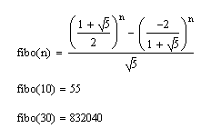
Also included in the module is a formula for computing Fibonacci numbers directly, without summing a lot of terms. J. P. M. Binet (1786-1856) conventionally gets credit for finding it first (it's called the Binet formula), although A de Moivre (1667-1754) knew about it earlier. I became aware of this formula in correspondence with David Zachmann, who derived it independently in the context of his own investigations.

image


Independent rediscovery is very typical in mathematics, goes with the territory. Your students should feel validated and encouraged when their own reasoning powers bring them to discoveries already celebrated in the literature.

# useful constants (used in fibo3)
root5   = 5.0**0.5
gold    = (1+root5)/2.0 # same as phi, named to not conflict with phi()
tau     = 1/gold

def fibo3(n): # thanks to David Zachmann
    # return nth fibonacci number as a floating point
    return (gold**n - (-tau)**n)/root5)
An interesting fact about the Fibonacci numbers is that the further out you go, the closer fib(n+1)/fib(n) approaches to the golden ratio, symbolized by the Greek letter image (i.e. phi, pronounced fie).
>>> float(series.fibo(41))/series.fibo(40)
1.61803398875
>>> (1+5**0.5)/2
1.61803398875

We will encounter phi in many of our geometric studies, including in the next section of this essay. It's value may also be expressed as a continued fraction of the form:

             Phi = 1 + 1
                       -----
                       1 + 1
                           -----
                           1 + 1
                               ----
                               1 + ...

Continued fractions give us more opportunities to explore recursive function definitions. Here is one for computing Phi as a continued fraction to a user-supplied level of depth:

def phi(depth):
    if depth>0: 
       return 1.0 + 1.0/phi(depth - 1)
    else:
       return 1.0

The following excerpt from a command line session demonstrates usage:

>>> series.phi(1)
2.0
>>> series.phi(2)
1.5
>>> series.phi(3)
1.66666666667
>>> series.phi(50)
1.61803398875

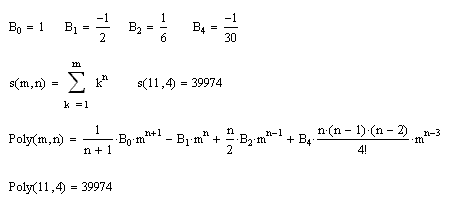
Another famous series of numbers is the Bernoulli series, named for Jacques Bernoulli (1654-1705) -- one of several powerful mathematicians in Bernoulli family. The Bernoulli numbers crop up all over in mathematics, including in the coefficients of polynomials of degree n+1 giving the sum of consecutive integers to the nth power.

For example, below is a summation of m consecutive integers to the 4th power, with a corresponding 5th degree polynomial. This polynomial will give the right answer for any integer m>0, as long as we keep n=4.

image

Like the Fibonaccis, we may derive the Bernoulli numbers with reference to the elements in Pascal's Triangle. Each successive row gives us the next fraction in the sequence (every Bernoulli number is a rational number, i.e. may be expressed in the form p/q).

def bernoulli(n):
    """
    Using rows from pascal's triangle, prow(n) in series.py:

     Bn = Bernoulli #       prow(n)
    ===============================
     1                       row 0
     1 1                     row 1
     1+2B1               =0  row 2
     1+3B1+ 3B2          =0  row 3
     1+4B1+ 6B2+4B3      =0  row 4
     1+5B1+10B2+10B3+5B4 =0  row 5
     ...
    """
    if n<=len(_bern):
        return _bern[n]   
    for k in range(len(_bern)+1,n+2):
       row = prow(k)
       nxtbern = -reduce(add,map(mul,_bern[:k-1],row[:k-1]))/row[-2]
       _bern.append(nxtbern)
    return _bern[n]

The algorithm first checks the cache to see if we already have B(n) on file. If not, we extend our list, picking up from the last Bernoulli number in _bern, and using successive rows from Pascal's Triangle to compute successive Bernoullis. Simply sum all the terms to the left of the still-unknown Bernoulli, negate it (i.e. bring it to the other side of the equation), and divide by the coefficient of the unknown. For example: B4 = -(1 + 5B1 + 10B2 + 10B3)/5. Here are the first 10 Bernoullis -- note that the odd Bernoullis are all 0 after B1.

>>> map(series.bernoulli,range(1,11))
[-1.0/2.0, 1.0/6.0, 0.0/1.0, -1.0/30.0, 0.0/1.0, 1.0/42.0, 0.0/1.0, 
-1.0/30.0, 0.0/1.0, 5.0/66.0]

The series.poly function will generate the terms of an n+1 degree polynomial corresponding to the sum of m consecutive integers raised to the nth power, while series.evalpoly will evaluate and add these terms. We can use series.sigma to cross-check the result. For example:

>>> terms = series.poly(15)   # sum of 1...m each raised to 15th power
>>> terms
['(1.0/16.0)*m**16', '(1.0/2.0)*m**15', '(5.0/4.0)*m**14', 
'(-91.0/24.0)*m**12', '(143.0/12.0)*m**10', '(-429.0/16.0)*m**8', 
'(455.0/12.0)*m**6', '(-691.0/24.0)*m**4', '(35.0/4.0)*m**2']
>>> series.evalpoly(terms,11) # computing the sum for m=11
5423573025795276.0
>>> series.sigma(11,15)       # cross-check 
5423573025795276L

Ada Byron (1815-1852) daughter of the poet Lord Byron, collaborated with Charles Babbage (1791-1871) on early designs for a programmable calculating machine. Her paper on how the Babbage difference engine might be used to compute Bernoulli numbers earned her the title of "first computer programmer" and the USA Defense Department named the Ada computer language in her honor in 1980.

For further reading:

Computer Language Resources


oregon.gif - 8.3 K
Home Page